Step by step tutorial

In this example we will guide you to the first use of the hardware setup. The neural network we will build has the following structure:

• a population of 50 neurons
• a DVS sensor that sends excitatory input to the population

We will assume the hardware setup is on and working properly. If this is not the case, please refer to the hardware section of the documentation.

Import

import pyNCS

That’s it.

Loading a setup

With setup we refer to the set of chips, boards, mapper, server, clients... everything that is used in the hardware experiment. To control the setup we implemented a pyNCS.NeuroSetup class. First copy the contents of chipfiles, biases and setupfiles directory from the pyNCS module to a local folder where you want to the experiments. Then run:

#Specifies the path to the setupfiles directory
setupdir = './setupfiles/'
#Constructs the nsetup object.
nsetup = pyNCS.NeuroSetupAPI(setupdir+'zenzero_setuptype.xml',
                          setupdir+'zenzero.xml',
                          prefix='./'
                          )

The setup is needed to create all the elements of the experiment, such as populations, connections, stimuli etc. It encapsulates all the informations about the hardware used. These informations are contained in xml files.

The first xml file contains the setuptype. In this example, the setuptype is a setup with 4 AER channels: 4 chips can be connected in a loop. The second xml file contains informations about which chip is connected to which AEX board and which AMDA board. These informations are needed by the system to access chips, i.e. get/set biases, send/receive as well as encode/decode AER events, get/set mapping tables implementing the connectivity of the network, etc. (see Software Installation for more details).

Note

If you run through the network, which means for this tutorial any computer besides zenzero, then you must have an account on zenzero and copied your public key to it. You can conveniently do this with:

ssh-copy-id -i ~/.ssh/id_rsa.pub username@zenzero

For example, to get all the parameters of a chip:

parameters = nsetup.chips['ifslwta0'].get_parameters()

Note

In case there are problems in loading the setup, you may want to take a look at :doc: to fix or prevent errors.

Creating populations

A population is a group of neurons on a chip. Each chip contains a certain number of neuronal circuits (somata). Each neuron has a certain number of synapses. If the chip is a neuromorphic sensor, it is very unlikely to have synapses...

Let’s create a population of neurons:

my_pop = pyNCS.Population( 'my_pop', 'My first population')

The population is empty until we populate it, which means we have to fill it up:

my_pop.populate_by_number( nsetup, 'ifslwta0', 'excitatory', 50)

There are several ways of populating. In this example we don’t care about the position of the neurons on the chip, we just want to use 50 neurons. To do this, we called the populate_by_number function with the following arguments:

• nsetup: the setup
• 'ifslwta0': this is the name of the chip containing the neurons we want to use
• 'excitatory': in a neuromorphic chip there are in general several groups of neurons, sharing biases, connectivity or other properties. We have to tell the system which one of these groups we want to pick-up neurons from.
• 50: the number of neurons we need

Neurons and synapses are represented as digital addresses. This means that the population is basically a container of addresses.

Let’s create the input population:

input_pop = pyNCS.Population('input', 'Virtual input neurons')
input_pop.populate_by_number(nsetup, 'seq', 'excitatory', 100)

The virtual chip ‘seq’ has 4096 neurons, but the corresponding population will have 100 neurons. You can check this by typing:

len(input_pop) #Should output 100

Setting parameters

Each chip has a certain amount of parameters that can be set. Parameters are mostly biases and we can control them by changing gate voltages of the corresponding transistors. Normally there is a voltage that controls the leak of the neuron, one that controls the weight of the excitatory synapses, one for the time constants, and so on and so forth. Before starting any experiment with the hardware one has to set the biases, which more or less corresponds to the boot operation of traditional computers.

The relation between a voltage and the corresponding physical quantity that it controls is what is called parameter translation. There are several theoretical and empirical methods that try to operate this translation in a systematic and reliable way in order to adjust the parameters to each experiment. We will not cover the problem here and will assume you are already in possess of basic sets of biases. What this practically means is explained as follows.

The set of parameters can be very large. Usually we handle this parameters using text files. We already have bias files for default sets of parameters for basic experiments but each experiments has usually its own set. Most probably you have already copied the biase files into the biases folder. Now you would like to load this biases to boot the system in the proper configuration. The operation is as simple as the following:

nsetup.chips['ifslwta0'].load_parameters('biases/ifslwta_default.biases')

Note

The DVS sensor doesn’t have digital biases but physical potentiometers on the board it is soldered on. Do not change them unless you know what you are doing.

Creating connections

We now need to connect the sensor output the excitatory synapses of our population of 50 neurons. This will be done using the pyNCS.Connection class:

C = pyNCS.Connection(input_pop, my_pop, 'excitatory0', 'all2all')

The excitatory0 string is the name of the excitatory synapses the each neuron of the ifslwta0 chip has. The last argument is the connectivity fashion, the default one is a one-to-one connectivity. With an all-to-all connectivity, our 50 neurons will represent the average activity of the whole input array.

Note

There is also a lower level pyMap module which also has a very nice interactive GUI. You may want to use it to check that the mapping is correct. (As of Jan 2012, pyMAP is broken). Try the following:

mapper_hostname = 'zanzara2' # change this to the real hostname!
M = pyMap.Mapping(setup, host=mapper_hostname).gui()
M.mainloop()

Sending and receiving stimuli

In some experiments you want to interact in real-time with the system. For example, you might have sets of recordings of calcium concentrations that you want to convert into spikes and send to the system. Here we will show how to send and receive events from the hardware.

Suppose you have vectors of mean-rates of a population of neurons. You can now create poisson trains with constant mean-rates corresponding to those of your vector. Let’s than turn off the DVS (power off) to replace the real-time input with the input we will send to the system.

There are several functions to create trains of spikes. These functions are usually methods of the population.soma group.

from numpy import random
#Generate a list of random numbers uniformly distributed in [20,30]
meanrates = random.random(len(input_pop))*10 + 20

stim = input_pop.soma.spiketrains_poisson(meanrates, duration=2000)

The variable stim now contains our spike-trains (a SpikeList instance from pyST.spikes) with poisson trains of random mean-rates between 20Hz and 30Hz lasting for 2000ms.

By default, the input synapse ‘excitatory0’ is initially turned off by setting its weight to zero. You can increase the weight by setting the appropriate bias as follows:

nsetup.chips['ifslwta0'].set_parameter('nsynstdw0',0.4)

We can not send the input and monitor some output using nsetup.run:

output = nsetup.run(stim)

Note

If you are using the ‘pyAex.api.com_aextcpclient’ as the communicator (see Software Installation), you must be sure that the server is started on the host:

#Go to your pyAex direction in a shell on the host computer
cd pyAex/Script/
#Start the server
python Server.py

To stop the server, type stop

Monitors and plots

There are several ways to visualize spiketrains. Assuming stim is a SpikeList object, the most basic vizualization is as follows:

from pylab import ion
ion()

stim[input_pop.soma.channel].raster_plot()

output[my_pop.soma.channel].raster_plot()

Monitors are a much more convenient way of visualizing data when dealing with several populations of neurons. A monitor will slice addresses and times according to the Population it is monitoring.

Create a monitor with the following:

from pyNCS.monitors import SpikeMonitor
my_mon = SpikeMonitor(my_pop.soma)

Then import it to the setup with:

nsetup.monitors.import_monitors([my_mon])

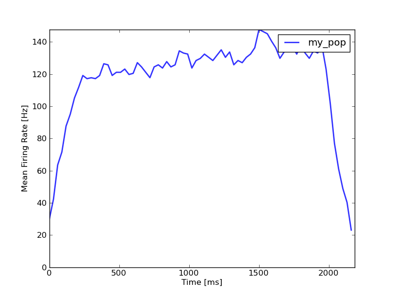
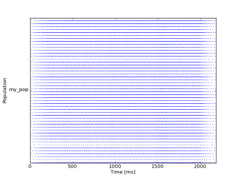
When nsetup.run is run, my_mon gets automatically populated with the relevant output spikes. You will have to run nsetup.run again or nsetup.monitors.populate_monitors(output). Raster plots and rate plots can be convienently obtained with:

from pyNCS.monitors import RasterPlot, MeanRatePlot
RasterPlot(my_mon)
MeanRatePlot(my_mon)

The results should look like this:

You can also use SpikeMonitors to vizualize inputs:

input_mon = SpikeMonitor(input_pop.soma)
input_mon.populate(stim[input_pop.soma.channel])
RasterPlot(input_mon)
MeanRatePlot(input_mon)

Beyond this tutorial

Congratulations, you have completed the first NCS tutorial and began your neuromorphic hardware career. If you want to see furhter examples, download the zenzero_unittest folder from the svn repository https://svn.ini.uzh.ch/repos/ncs/ini/code/python/ncs_unittests/zenzero_unittest, and take a look at the folders in the test directory. Each test can be run independently by typing:

cd tests/test_swta_ifslwta0
ipython
run expRun

The entire unittests can be run with:

python zenzero_unittest.py