The Python Oscilloscope Module

written on 2/12 2010 by Andreas Steiner

Introduction

This package provides the Oscilloscope class which actually is an abstraction wrapper that can be used to access any oscilloscope-like device for which exists a ‘driver’. So far there is only a driver provided for the Spectrum Card – Normally you wouldn’t care too much about the actual drivers and only use the wrapper. Using a different oscilloscope then results in a simple change of one line of code:

from pyOsc.spectrum import SpectrumCard as driver # already implemented
# from pyOsc.agilent import AgilentEthernetController as driver # not yet implemented !

import pyOsc
osc= pyOsc.Oscilloscope( driver() )

Tutorial

Initializing

Let’s assume we are connected via ssh to zaex where the SpectrumCard is currently installed and let’s assume we have some single chip setup as described in the setup file zaex.xml

import pyOsc,pyNCS
from pyOsc.spectrum import SpectrumCard as driver # already implemented
osc= pyOsc.Oscilloscope( driver(debug=True) )
basedir = '/home/federico/pyFED/'
setup = pyNCS.NeuroSetup(basedir+'setups/mc_setuptype.xml',basedir+'setups/mc.xml');

The spectrum card has 8 channels. As of the time of writing this tutorial, we have them connected to the ifslwta chip in a particular way. In order to avoid confusing the lines and signals, we can label the channels like this

osc.names( {
0 : 'Vmem127',
1 : 'Vsyn ("Vpls")',
2 : 'Vpls ("Vsyn")',
3 : 'VsynAER',
4 : 'VplsAER',
5 : 'Vk',
6 : 'Vwstd',
7 : 'Vmem (scanner)' })

Getting some data

In the simplest scenario, we inject some current, set the scanner to any neuron, setup the channels and just start recording

osc.channels( [7] ) # activate only 1 channel
osc.ranges( {7:1000} ) # set the range to (-1000mV) to (1000mV)
osc.sr( 1024 ) # sample rate in Hertz
setup.find('ifslwta').bias.pinj.v= 2.87 # inject some current into all neurons

We know that all the neurons are firing more or less continuously due to the injection current. We would like to acquire 5 seconds of data. The whole process of data acquiring is completely asynchronous, so we have to tell the oscilloscope how much data we would like and then we need to wait until the oscilloscope is ready:

samples= 5* osc.sr()
osc.start( samples )
import time
while not osc.done(): time.sleep(1)

When we got so far, the whole data is acquired and can be found on the oscilloscope. In order to process it in python scripts, we need first to transfer it to the computer memory. This is done by

data= osc.data()

The data is now contained in raw format in the dictionary data. The keys to the dictionary are the channel numbers and the samples are of type numpy.int16 (for the spectrumcard, other drivers may specify different sample types).

Visualizing the data

Simply type

osc.plot( data )
from matplotlib import pyplot as plt
plt.show() #pop up plot

This should result in a plot similar to the following

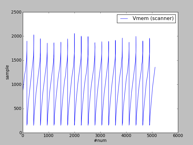
If you want to display the data in millivolt and milliseconds instead of samples, simply type

osc.plot( osc.normalize(data) )

Setting a trigger

Let’s suppose we want to have a nice picture of the spiking neuron. You can easily see in the figure above that the different spikes are not exactly the same, so let’s take the average over several cycles to get a smoother and more representative image.

In order to do this we will set a trigger on the sharp falling edge of the membrane potential and center the data around that trigger. Let’s first precisely determine the point we want to trigger at. For this purpose I use the normalized data plot from above, zoom a little bit closer and move my mouse cursor to the point I want to trigger at:

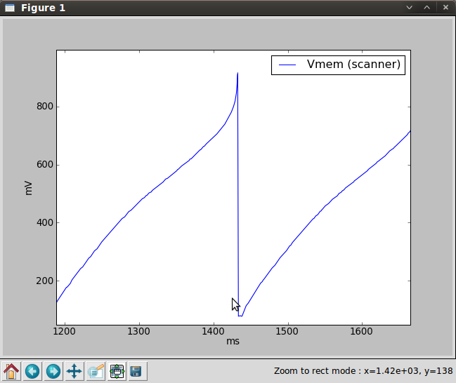
Ok. What we want is the following

• Trigger on the falling edge at 138 mV (on channel 7).
• Record 200ms on every trigger.
• Center the falling edge at 20% of these 200ms.
• Collect 10 ‘rounds’ of data.

This translates into the following code

osc.trigger( 7,'\\',138,offset=.2 )
samples= osc.sr() * .2
osc.rounds( 10 )

As above, we start the data acquisition, wait for the oscilloscope to be ready and transfer the data:

osc.start( samples )
import time
while not osc.done(): time.sleep(1)
data= osc.data()

The raw plott looks pretty confusing, because we the different rounds are just concatenated one after the other in the sample data. That’s why we let the oscilloscope wrapper plot markings between the rounds and indicate the trigger level with a red line

osc.plot( data,decorate=True )

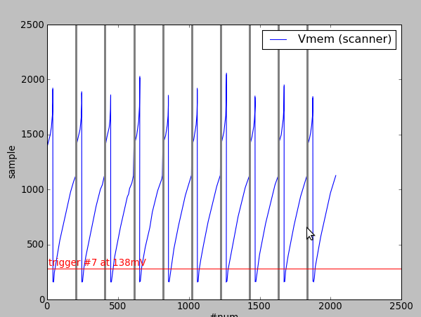
We can now calculate our smooth plot by averaging the rounds. There’s a convinience method in Oscilloscope to do this

average= osc.average(data)
osc.plot(osc.normalize( average ))

Feedback

If you found this tutorial useful or if you have any questions or if things did not work out the way they are supposed to, you can always send me an email